Macroscopic model for evacuation of bees
We investigate a Hughes model for controling the evacuation of Bees on a surface in 3D . The Hughes model is a system of partial differential equations (PDEs) and consists of a nonlinear transport equation and an Eikonal equation which determines the movement direction of Bees. Indeed, the Hughes model is a continuum macroscopic model which can be simulate the global movement effects by interpreting Bees as particles of flow. Considering this model, Bees tend to choose the shortest path (in a certain metric) to reach the outlet of beehive but it may be at a slower speed. To minimize the evacuation time and control the path of Bees through the outlet, we add a convection term (additional driving force) to the nonlinear transport equation.
Prelimineries
By defining
\[ \color{blue}{\beta := - v^2_{\max}(\rho) \nabla \phi} \]
as transport direction, we consider the following regularized Hughes model where the motion of crowds is modelled by PDEs\[ \partial_t \rho - \nabla \cdot (\rho \ v^2_{\max}(\rho) \nabla \phi) = \color{red}{\varepsilon} \Delta \rho,\] \[ - \color{red}{\delta_1} \Delta \phi + | \nabla \phi |^2 = \dfrac{1}{\color{green}{v_{\max}(\rho)^2} + \color{red}{\delta_2}}.\]
The model contains diffusion and Eikonal equations and is completed with the following initial and boundary conditions
\[ \rho(0,\cdot) = \rho_0 \qquad \text{in} \ \Omega \\ -(\varepsilon \ \nabla \rho + \rho \ v_{\max}(\rho)^2\ \nabla \phi) \cdot n = \tilde{v}_{\max} \ \rho \qquad \phi = 0 \qquad \text{on} \ \Gamma_{D}, \]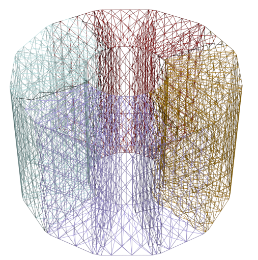
- The density function which represents a crowd \[ \rho\in C^1(0,t_n;C^2(\Omega)) \qquad \rho(t,\mathbf{x}): [0,t_n] \times \Omega \mapsto \mathbb{R} \]
- The potential for \( \mathbf{x} \in \Omega \subset \mathbb{R}^3 \) \[ \phi\in C^2(\Omega) \qquad \phi(t,\mathbf{x}): [0,t_n] \times \Omega \mapsto \mathbb{R} \]
- The chosen velocity model as \[ \color{grren}{v_{\max}}\in C^1(\Omega) \qquad v_{\max}(\rho) = 1- \rho \]
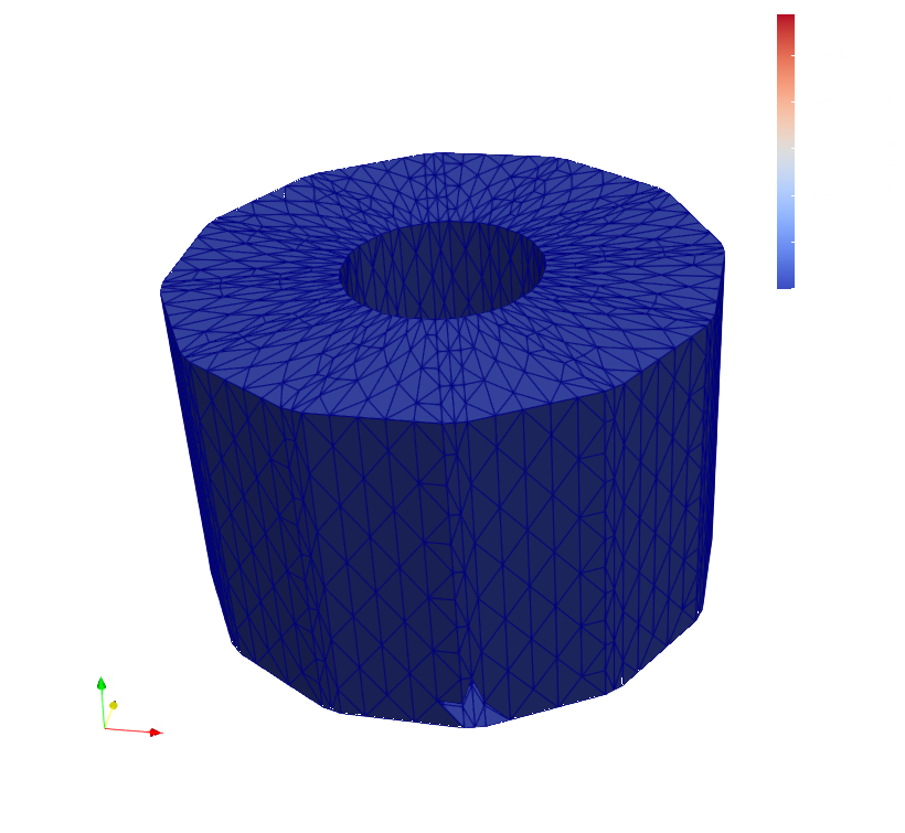
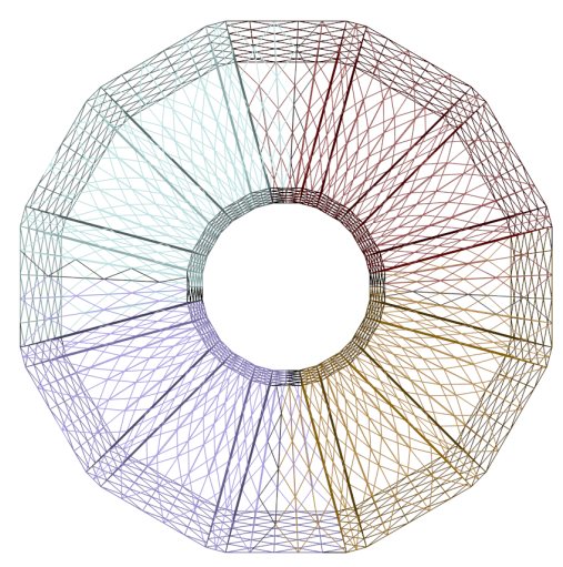
- \( \mathcal{T}_h : \) family of conforming triangulations over a domain \( \Omega \)
- The cell averages for element \( T \in \mathcal{T}_h \) \[ \bar{\rho}_{T} = |T|^{-1} \int_{T} \rho \ dx \]
Weak formulation
Let \( H^1_{D}(\Omega) = \{v \in H^1(\Omega): v|_{\Gamma_D} = 0 \} \) and Define: \[ V_h = \{ v \in L^{2}(\Omega): v|_{T} \in \mathcal{P}^{0}(T)\ \text{for all} \ T \in \mathcal{T}_h\},\\ W_h = \{ v \in C(\bar{\Omega}): v|_{T} \in \mathcal{P}^{1}(T)\ \text{for all} \ T \in \mathcal{T}_h\} \cap H^1_{D}(\Omega), \] Using the finite element method (FEM) for space discretizations, we aim to find \( \rho\in C^1(0,t_n; V_h) \) and \( \phi \in W_h \) such that \[ \int_{\Omega} \partial_t \rho\ v \ dx + \int_{\Omega}(\rho \ v^2_{\max}(\rho) \nabla \phi) \cdot \nabla v\ dx - \int_{\Gamma} (\rho \ v^2_{\max}(\rho) \nabla \phi) \cdot v\ dx -\varepsilon \int_{\Omega} \nabla \rho\ \nabla v \ dx + \varepsilon \int_{\Gamma} \nabla \rho\ v \ dx, \quad \forall v \in V_h \\ \delta_1 \int_{\Omega} \nabla\phi \ \nabla w \ dx + \int_{\Omega} | \nabla \phi |^2 \ w \ dx = \int_{\Omega} \dfrac{1}{v_{\max}(\rho)^2 + \delta_2}\ w \ dx, \quad \forall w \in W_h \] It can be rewritten as \[ \int_{\Omega} \color{purple}{\partial_t \rho}\ v \ dx +\varepsilon \Big(\int_{\Omega} \nabla \rho\cdot \nabla v \ dx - \int_{\Omega} \color{red}{[[ \nabla \rho ]]}\cdot [\![v]\!]_n dx - \int_{\Omega} \color{red}{[[ \nabla v ]]}\cdot [\![\rho]\!]_n dx + \frac{1}{h} \int_{\Omega} \color{green}{[\![\rho]\!] [\![v]\!]} dx\Big)+ \int_{\Gamma} \tilde{v}_{\text{max}}\ \rho\ v \ dx = - \int_{\Omega} \color{blue}{(\bar{\rho}\ \beta)} \cdot \color{green}{[\![v]\!]} \ dx, \quad \forall v \in V_h \]- Average of a function across a common facet of two cells: \( [[v]] = \frac{1}{2} (v^{+} + v^{-}) \)
- Jump of a function across a common facet of two cells: \( [\![v]\!] = v^{+} - v^{-},\)
- \( [\![v]\!]_{n} := v^{+}\cdot n^{+}+ v^{-} \cdot n^{-} \)
- Using Lax-Friedrich flux for the convective flux, \[ (\bar{\rho}\ \beta) = [[\bar{\rho}\ \beta]]\cdot n - \dfrac{\eta}{2} [\![\bar{\rho} ]\!],\] Finally, we use the finite difference (FD) method to discretize the temporal direction \[ \partial_t \rho \approx \dfrac{\rho^{n+1} - \rho^{n}}{\tau}, \qquad \tau = t_{n+1} - t_n.\]
Adding an additive convection term
We add an additive convection term to control the speed and direction of bees during exiting. Therefore, we have the following PDE with the initial and boundary conditions \[ \partial_t \rho - \nabla \cdot (\rho \ v^2_{\max}(\rho) \nabla \phi) \color{red}{+ \ \vec{v}_{\text{vel}} \nabla \rho} = \varepsilon \Delta \rho, \\ - \delta_1 \Delta \phi + | \nabla \phi |^2 = \dfrac{1}{v_{\max}(\rho)^2 + \delta_2}.\] Since \( \rho \in V_h \), then we have to use \(\frac{1}{h} [\![\rho]\!]_{-n} \) instead of \( \nabla \rho \) . Therefore, the variational formula regarding this case is as follows \[ \int_{\Omega} \partial_t \rho\ v \ dx +\varepsilon \Big(\int_{\Omega} \nabla \rho\cdot \nabla v \ dx - \int_{\Omega} [[ \nabla \rho ]]\cdot [\![v]\!]_n dx - \int_{\Omega} [[ \nabla v ]]\cdot [\![\rho]\!]_n dx + \frac{1}{h} \int_{\Omega} [\![\rho]\!] [\![v]\!] dx\Big)+ \color{red}{\frac{1}{h} \int_{\Gamma} \vec{v}_{\text{vel}} \cdot( [\![\rho]\!]_{-n}\ [[v]]) \ dx} + \int_{\Gamma} \tilde{v}_{\text{max}}\ \rho\ v \ dx \\ \qquad \qquad \qquad= - \int_{\Omega}(\bar{\rho}\ \beta) \cdot [\![v]\!] \ dx, \quad \forall v \in V_h \\ \delta_1 \int_{\Omega} \nabla\phi \ \nabla w \ dx + \int_{\Omega} | \nabla \phi |^2 \ w \ dx = \int_{\Omega} \dfrac{1}{v_{\max}(\rho)^2 + \delta_2}\ w \ dx, \quad \forall w \in W_h\]
Main Overview
To apply the Hughes model to the surface mesh of the beehive, three steps are required:
- Define geometry and meshing
- Geometry definition
- Doors for exiting Bees
- Rectangular cube
- Converting an STL file to XDMF file
- Reading XDMF file in python